The other day I received the following message:
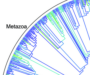
“I'm using your R package phytools to plot a circular tree
(contMap function), but I'd like to annotate the family names
outside the tree, just like the example file attached. I have looked for it in
your blog and on internet, but I did not find anything similar with a code
available. Is this possible to do with phytools?”
In which the following is a snippet of her example:
This does not exist in R, so far as I know. However, the package plotrix, already imported by phytools, has a number of cool functions that I thought might be useful to achieve this effect.
First, here is my (beta) function:
arc.cladelabels<-function(tree=NULL,text,node,ln.offset=1.02,
    lab.offset=1.06,cex=1,orientation="curved",...){
    obj<-get("last_plot.phylo",envir=.PlotPhyloEnv)
    if(obj$type!="fan") stop("method works only for type=\"fan\"")
    h<-max(sqrt(obj$xx^2+obj$yy^2))
    if(hasArg(mark.node)) mark.node<-list(...)$mark.node
    else mark.node<-TRUE
    if(mark.node) points(obj$xx[node],obj$yy[node],pch=21,
        bg="red")
    if(is.null(tree)){
        tree<-list(edge=obj$edge,tip.label=1:obj$Ntip,
            Nnode=obj$Nnode)
        class(tree)<-"phylo"
    }
    d<-getDescendants(tree,node)
    d<-sort(d[d<=Ntip(tree)])
    deg<-atan(obj$yy[d]/obj$xx[d])*180/pi
    ii<-intersect(which(obj$yy[d]>=0),which(obj$xx[d]<0))
    deg[ii]<-180+deg[ii]
    ii<-intersect(which(obj$yy[d]<0),which(obj$xx[d]<0))
    deg[ii]<-180+deg[ii]
    ii<-intersect(which(obj$yy[d]<0),which(obj$xx[d]>=0))
    deg[ii]<-360+deg[ii]
    draw.arc(x=0,y=0,radius=ln.offset*h,deg1=min(deg),
        deg2=max(deg))
    if(orientation=="curved")
        arctext(text,radius=lab.offset*h,
            middle=mean(range(deg*pi/180)),cex=cex)
    else if(orientation=="horizontal"){
        x0<-lab.offset*cos(median(deg)*pi/180)*h
        y0<-lab.offset*sin(median(deg)*pi/180)*h
        text(x=x0,y=y0,label=text,
        adj=c(if(x0>=0) 0 else 1,if(y0>=0) 0 else 1),
        offset=0)
    }
}
library(phytools)
library(plotrix)
tree
##
## Phylogenetic tree with 100 tips and 99 internal nodes.
##
## Tip labels:
##  t1, t7, t25, t26, t2, t3, ...
##
## Rooted; includes branch lengths.
nodes<-c(104,118,122,137,149,175,189,190)
labels<-paste("Clade",LETTERS[1:length(nodes)])
plotTree(tree,type="fan",lwd=1,ftype="off",xlim=c(-1.1,1.1))
for(i in 1:length(nodes))
    arc.cladelabels(text=labels[i],node=nodes[i])

Maybe we notice that for two of the clades there is not really enough space to plot their labels circularly, and would rather plot them horizontally. We can do this too:
plotTree(tree,type="fan",lwd=1,ftype="off",xlim=c(-1.1,1.1))
for(i in 1:length(nodes))
    arc.cladelabels(text=labels[i],node=nodes[i],
        orientation=if(labels[i]%in%c("Clade B","Clade G"))
        "horizontal" else "curved")

If we want to include tip labels in the plot we will need to adjust
the two arguments ln.offset and lab.offset,
which are specified as a multiplier of total tree depth. You may also notice
that the clades to be labeled have their MRCA noted with a red dot. We can
turn this off easily.
plotTree(tree,type="fan",lwd=1,ftype="i",fsize=0.7,xlim=c(-1.2,1.2))
for(i in 1:length(nodes))
    arc.cladelabels(text=labels[i],node=nodes[i],ln.offset=1.1,
    lab.offset=1.15,mark.node=FALSE)

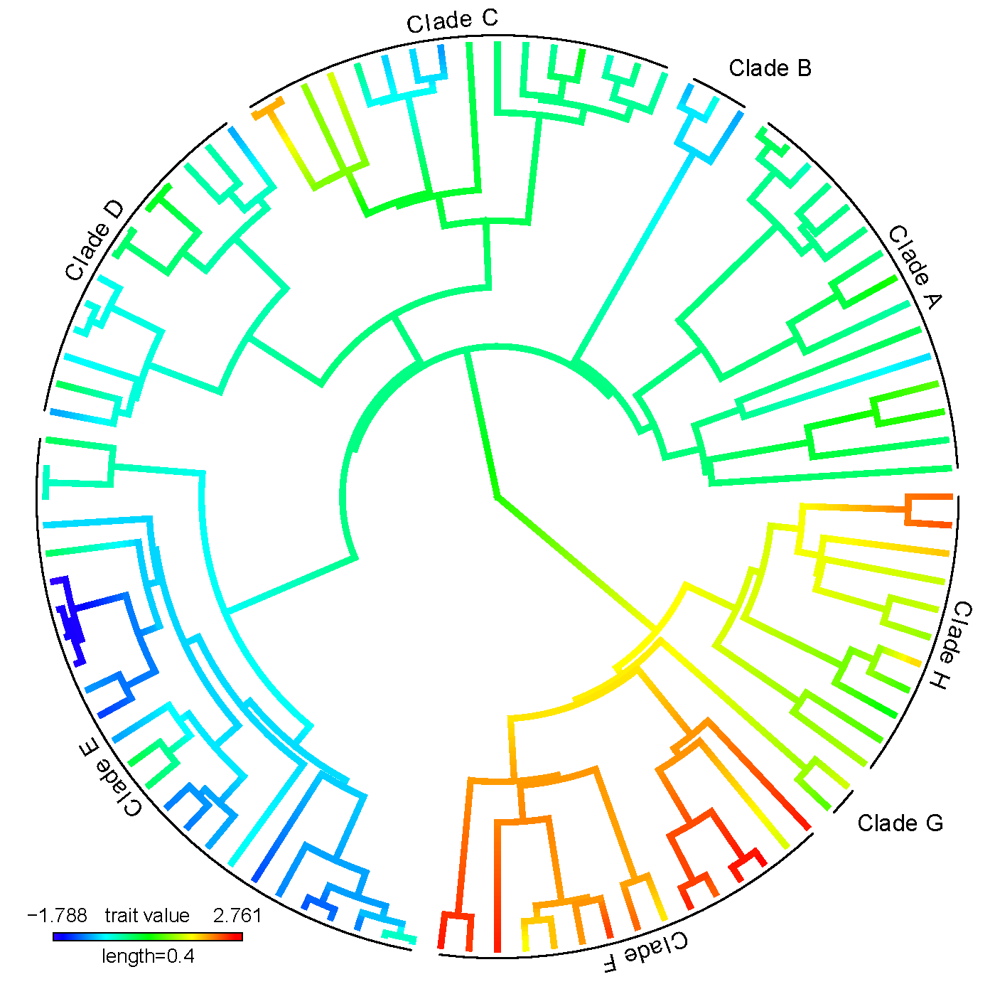
Finally, it is straightforward to use this with other plotting methods,
such as plot.simmap or plot.contMap. For instance:
x
##           t1           t7          t25          t26           t2
##  0.185429207  0.094608262  0.760719557  0.963119247 -0.613742776
##           t3          t13          t30          t31          t35
##  0.248102131 -0.118475199  0.694191486  0.071582483  0.050032594
##          t50          t51          t70          t86          t87
##  0.032262629 -0.001892491 -0.229326634  0.283981779  0.164694487
##          t32          t71          t72          t55          t76
## -0.861695430 -0.352169565 -0.797383594 -0.147875574  0.059193790
##          t77          t66          t67          t34          t22
## -0.236570859  0.523480198 -0.055877020 -0.012512494  0.128464862
##           t4          t64          t65          t48          t49
##  0.213153746 -0.928063215 -0.648886144 -0.684025531  0.006881137
##          t15          t16          t91          t92          t21
##  1.523355788  1.218056983  2.038305894  2.019228156 -0.851746986
##          t38          t39          t99         t100          t95
## -0.119677916 -0.090495321  0.444701776  0.445875273  0.189022674
##          t96          t73          t82          t83          t20
##  0.067742383 -0.423314363 -0.371488270 -0.406287550 -0.512160615
##          t28          t29          t24          t97          t98
##  0.247582627 -0.879421691  0.221554029 -0.227690642 -0.242492947
##          t14          t17          t81          t89          t90
## -0.627299910  0.187249019 -1.788281688 -1.673693103 -1.608081213
##          t88          t58          t59          t27          t56
## -1.736842698 -0.924691207 -1.313277929 -0.878893215  0.317057217
##          t57          t62          t63          t52          t11
##  0.146722922 -1.035700313 -1.042831693 -0.853733850 -0.427358894
##           t9          t33          t84          t85          t78
## -1.257660829 -0.990611837 -1.239630360 -1.095542278 -1.063870076
##          t93          t94          t60          t61           t8
## -0.144898325 -0.436375725  2.675756270  2.523984420  2.657743208
##          t68          t69          t53          t54          t40
##  1.632048013  1.937727602  2.119883643  2.527910126  2.344777813
##          t41          t74          t75          t79          t80
##  1.762067736  2.630088860  2.361542350  2.651599024  2.761170468
##           t6           t5          t46          t47          t18
##  1.519560349  2.667583940  0.945310915  1.491948899  1.299554468
##          t19          t23          t44          t45          t36
##  0.902194960  0.497576835  0.834872192  1.858746870  1.234396753
##          t37          t12          t10          t42          t43
##  1.425951772  1.439553510  1.922945651  2.420284774  2.341460432
obj<-contMap(tree,x,plot=FALSE)
obj<-setMap(obj,invert=TRUE) ## invert color map
plot(obj,ftype="off",type="fan",outline=FALSE,legend=0.4,
    fsize=c(0,0.8))
for(i in 1:length(nodes))
    arc.cladelabels(text=labels[i],node=nodes[i],
        orientation=if(labels[i]%in%c("Clade B","Clade G"))
        "horizontal" else "curved",mark.node=FALSE)

(Non-aliased version here.)
Some bugs to iron out, no doubt - but not bad!
This comment has been removed by the author.
ReplyDeleteLiam, this clade labels are fantastic! But, I wonder if there is a possible way to determine clades by the tips (instead of by the nodes), since some clades could have just one branch.
ReplyDeleteAll the best,
- Carlos Biagolini-Jr.
Hi Carlos. I just posted a solution here. Let me know if this helps. - Liam
DeleteThank you Liam, it opens new possibilities to display phylogenetic data!
ReplyDelete- Carlos
It would be good to have the lab.offset in cladelabels too
ReplyDelete