Overlaying a posterior density map from stochastic mapping on your phylomorphospace

Thinking about phylomorphospaces for the first time in a bit last night, when I realized that we can now use phytools to pretty easily overlay a posterior density map from stochastic mapping (e.g., here) onto a projection of the tree into two dimensional morphospace - i.e., a phylomorphospace plot (e.g., here). This is how we do it.

First, for the purposes of demonstration, let's simulate some data with a high rate & correlation between x & y when our simulated discrete character is in the derived state '1', and a low rate & correlation when in the ancestral state '0':

> # simulate tree & data
> Q<-matrix(c(-1,1,1,-1),2,2)
> rownames(Q)<-colnames(Q)<-c(0,1)
> tree<-sim.history(pbtree(n=40,scale=1),Q,anc="0")
> R<-list(matrix(c(1,0,0,1),2,2),matrix(c(2,1.8,1.8,2), 2,2))
> names(R)<-c(0,1)
> X<-sim.corrs(tree,R)
> colnames(X)<-c("x","y")

Next, let's conduct empirical Bayes stochastic mapping & then generate a posterior density map:

> # Ok, now do stochastic character mapping
> mtrees<-make.simmap(tree,tree$states,nsim=100, message=FALSE)
> # densityMap
> dmap<-densityMap(mtrees)
sorry - this might take a while; please be patient

Finally, let's overlay the density map on our phylomorphospace plot:

> phylomorphospace(dmap$tree,X,colors=dmap$cols, node.by.map=TRUE,xlim=c(-1.7,2))
> add.simmap.legend(colors=setNames(c(dmap$cols[1], dmap$cols[length(dmap$cols)]),c(0,1)))
Click where you want to draw the legend

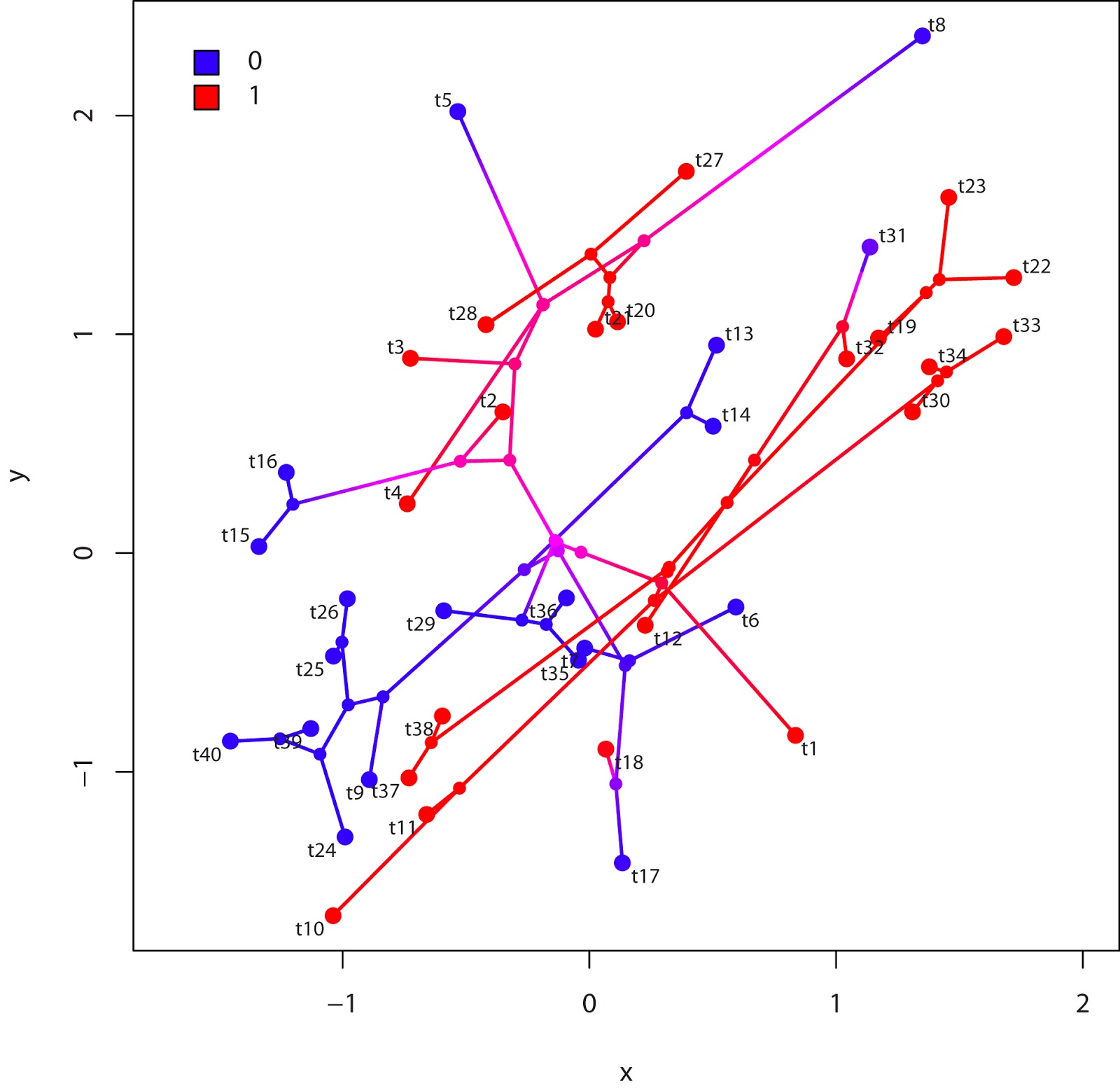
Pretty cool.