New phylo.to.map with direct projection of the tree onto a geographic map

A few days ago I added the option to directly project a phylogeny onto a geographic map into the S3 method plot.phylo.to.map. The most recent phytools version (phytools 0.3-20) is available from my website. It also allows the use of alternative map databases and maps. Here's a quick demo:

> require(phytools)
Loading required package: phytools
> packageVersion("phytools")
[1] ‘0.3.20’
> require(mapdata)
Loading required package: mapdata
> xx<-phylo.to.map(tree,cbind(lat,long), database="worldHires",plot=FALSE)
objective: 286
...
objective: 76
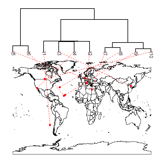
> # first, let's plot the phylogram visualization
> plot(xx,type="phylogram",asp=1.3)

> # now let's do a direct projection
> plot(xx,type="direct",asp=1.3)

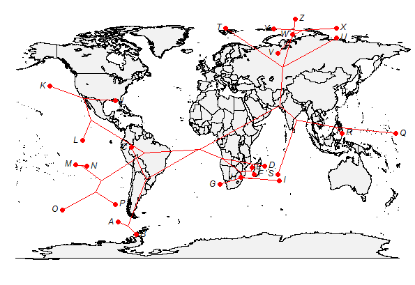
As before, it is a good idea to keep in mind that the nodes in the direct projection do not mean to show ancestral area reconstruction - they are just an attribute of the projection to show relationships among species.

New phytools version with some phylogeny & geographic mapping options

I'm new to geographic maps (see 1, 2), but they are fun to play with so, after a little work, I've added the function phylo.to.map. It now creates an object of class "phylo.to.map" which can be used with the S3 plotting method plot.phylo.to.map. The function also allows optional user control of a bunch of different plotting options; however these are not yet thoroughly documented.

The new version of phytools with these updates (phytools 0.3-19) also depends on the R package maps.

Here's a quick demo:

> require(phytools)
Loading required package: phytools
> packageVersion("phytools")
[1] ‘0.3.19’
> # simulate tree & data
> tree<-pbtree(n=26,scale=100)
> tree$tip.label<-LETTERS[26:1]
> lat<-fastBM(tree,sig2=10,bounds=c(-90,90))
> long<-fastBM(tree,sig2=80,bounds=c(-180,180))
> # now plot projection
> phylo.to.map(tree,cbind(lat,long),asp=1.3)
objective: 168
...
objective: 78

We can also zoom in on particular regions of the map, although that is not well developed. So, for instance:

> tree<-pbtree(n=26,scale=100)
> tree$tip.label<-LETTERS[26:1]
> lat<-fastBM(tree,sig2=10,bounds=c(-36,-16),a=-20)
> long<-fastBM(tree,sig2=80,bounds=c(115,150),a=130)
> # now plot projection
> phylo.to.map(tree,cbind(lat,long),ylim=c(-40,-10), xlim=c(110,155))
objective: 166
...
objective: 114

It's also now possible to project the tree directly onto a geographic map. Users of this method, though, should keep in mind that "ancestral nodes" are just a projection of the tree - and are not intended as a reconstruction of ancestral areas:

> tree<-pbtree(n=26,scale=100)
> tree$tip.label<-LETTERS[26:1]
> tree<-paintSubTree(tree,length(tree$tip)+1,"1")
> lat<-fastBM(tree,sig2=10,bounds=c(-90,90))
> long<-fastBM(tree,sig2=80,bounds=c(-180,180))
> plot.new()
> plot.window(xlim=c(-180,180),ylim=c(-90,90),asp=1.3)
> map("world",add=TRUE)
> phylomorphospace(tree,cbind(long,lat), colors=setNames("red",1),node.by.map=TRUE,add=TRUE, label="horizontal")

Addendum to plotting a tree linking tips to a global map

This isn't how I need to be spending my time (with an NSF grant due next week), but here's a neat addendum to my earlier post about a function to link the tips of a tree to plotted lat/long locations on a global map.

In that post I completely ignored the fact that all the links tend to cross each other because the tips of the tree have not been rotated to maximize the concordance of their order with the longitudinal position of the corresponding coordinates. Here is a function that attempts to do this via one pre-order tree traversal:

minRotate<-function(tree,x){
  tree<-reorder(tree)
  nn<-1:tree$Nnode+length(tree$tip.label)
  x<-x[tree$tip.label]
  for(i in 1:tree$Nnode){
    tt<- tt<-read.tree(text=write.tree(rotate(tree,nn[i])))
    oo<-sum(abs(order(x[tree$tip.label])-
     1:length(tree$tip.label)))
    pp<-sum(abs(order(x[tt$tip.label])-
     1:length(tt$tip.label)))
    if(oo>pp) tree<-tt
    message(paste("objective:",min(oo,pp)))
  }
  return(tree)
}

All that's going on in this incredibly simple function is that the function climbs from the root up through the nodes of the tree. It rotates each one and then checks to see if the objective function (the match in ordering between the tips of the tree and longitudinal coordinates in vector x) improves. It accepts only changes that decrease the value of the objective function.

This strikes me as a search algorithm that would have an incredible propensity to get stuck on local optima - but let's not speculate, let's give it a try. A new option in phylo.to.map optionally uses this optimization function internally.

> library(phytools)
> library(rworldmap)
### Welcome to rworldmap ###
...
> source("phylo.to.map.R")
> # simulate tree & data
> tree<-pbtree(n=26,scale=100)
> tree$tip.label<-LETTERS[26:1]
> lat<-fastBM(tree,sig2=10,bounds=c(-90,90))
> long<-fastBM(tree,sig2=80,bounds=c(-180,180))
> # first, unrotated
> phylo.to.map(tree,cbind(lat,long),rotate=FALSE)

> # now rotated
> phylo.to.map(tree,cbind(lat,long))
objective: 118
objective: 112
...
objective: 96

Well, that may not be perfect - but it is clearly a heck of an improvement. Let's try it again to make sure it wasn't a fluke:

> # simulate tree & data
> tree<-pbtree(n=26,scale=100)
> tree$tip.label<-LETTERS[26:1]
> lat<-fastBM(tree,sig2=10,bounds=c(-90,90))
> long<-fastBM(tree,sig2=80,bounds=c(-180,180))
> # first, unrotated
> phylo.to.map(tree,cbind(lat,long),rotate=FALSE)

> # now rotated
> phylo.to.map(tree,cbind(lat,long))
objective: 280
objective: 136
...
objective: 96

Cool. It can't be any worse than leaving the tree unrotated, anyway.

Connecting the tips of a plotted tree to coordinates on a map

A recent R-sig-phylo subscriber posted two questions (1, 2) about connecting the tips of a plotted tree to mapped lat/long coordinates on a global map. He was certainly on the right track, but I just posted a better solution (code for the full function, here). I don't have too much time to get into the details on how this was done, but it uses code from my simple tree plotter (with x & y flipped, of course); and plot the map & tree in the same plotting object.

Here is an example of a result from a simulated tree & the submitted lat & long coordinates of the R-sig-phylo reader:

Because this was the user request, and I don't have much time to work on this kind of stuff this week - I have only created this plotter to use a full, global map; however, it would be pretty straightforward (I think) to generalize it to an arbitrary map by pulling the map coordinates from the map object in memory.

Plotting the variance among stochastic character maps on the tree

The phytools function densityMap can be used to visualize the posterior probability of a binary character on the nodes & edges on the tree obtained via stochastic character mapping. By default, this function uses a continuous color gradient from blue to red (with low posterior probability for state 1 in blue); thus purple colors indicate high uncertainty about the state of the character mapped on the tree.

I thought it might be interesting to visualize the variance (i.e., uncertainty) of our ancestral reconstruction directly. We can compute the variance in our posterior probability (which is just a proportion from the posterior sample) as p(1-p). Here is what this looks like:

First, simulate a tree & some data, and then perform stochastic mapping × 100:

> tree<-pbtree(n=30,scale=2)
> Q<-matrix(c(-1,1,1,-1),2,2)
> rownames(Q)<-colnames(Q)<-0:1
> x<-sim.history(tree,Q)$states
> mtrees<-make.simmap(tree,x,nsim=100)

Now we're ready for my somewhat hacky solution for plotting the variance among stochastic maps on the edges & nodes of the tree. Note that this requires the latest phytools build, phytools 0.3-13.

XX<-densityMap(mtrees,plot=FALSE)
aa<-colnames(XX$tree$mapped.edge)
tt<-XX$tree
# collapse each prob with the same variance into each other
for(i in 0:499){
 oo<-c(as.character(i),as.character(1000-i))
 nn<-as.character(i)
 chk<-oo%in%aa
 if(sum(chk)==2) tt<-mergeMappedStates(tt,oo,nn)
 else if(chk[2])
  for(j in 1:length(tt$maps))
   names(tt$maps[[j]])[which(names(tt$maps[[j]])==
   oo[2])]<-oo[1]
}
# compute the variances
p<-as.numeric(names(XX$cols))/(length(XX$cols)-1)
v<-(p*(1-p))[1:501]
XX$tree<-tt
# this is a hack
XX$cols<-setNames(as.vector(rbind(grey(v/0.25), grey(v/0.25))),as.vector(rbind(0:500,0:500)))
XX$lims<-c(0,0.25)
class(XX)<-"contMap"
# plot!
plot(XX)

OK, now let's compare the normal contMap plot with our "uncertainty" plot. First, here is the contMap plot:

Now here is the variance plot:

That's it.

Complex numbers in R and a new version of phyl.cca

I just posted a new version of phyl.cca (my function for phylogenetic canonical correlation analysis) that addresses the following error, which initially seemed very alarming:

> phyl.cca(tree,X,Y)
Error in ccs > 0 : invalid comparison with complex values

It turns out that part spectral decomposition (eigenanalysis) can result in very slightly negative eigenvalues, which result in complex numbers during some steps of the calculations of CCA. In later steps, the imaginary parts go to zero - but R keeps the class of a number as "complex" even if the imaginary part is zero.

To fix this, I merely check to see if all imaginary parts of the canonical correlations are zero, and (if so) set the canonical correlation to the real part of the number only:

if(all(Im(ccs)==0)) ccs<-Re(ccs)

This seems to have solved the problems.

This update is also in a new phytools build (phytools 0.3-11) which can be installed from source.

Bug in rerootingMethod for tree with node labels

I recently learned that the function rerootingMethod breaks for trees with node labels. This seems to be due to a bug in an internally called function, not in rerootingMethod itself and can be eliminated by just setting:

> tree$node.label<-NULL

That's it.

New phytools build (phytools 0.3-10) on CRAN

There is a new phytools build on CRAN, phytools 0.3-10. Some of the updates in this version include: plotting partial fan trees; full user control of plotting options in plotBranchbyTrait; a new function to rotate all nodes or a set of nodes; small updates to densityMap and contMap; a new phylognetic scatter plot plotting method; and new plotting options for the labels in phylomorphospace (1, 2).

It will probably take a few days for Windows & Mac OS binaries to be build and for the package to percolate through the CRAN repositories. Check it out!

A different easier way to overlay time since the root onto a phylomorphospace

I realized after describing a method to overlay time since the root onto a phylomorphospace plot using a color gradient - I realized that there is a much easier way to do the same thing using the phytools function make.era.map. (To include the color legend, you should download the latest phytols version: phytools 0.3-07.)

Here's how to do it:

> # load phytools
> library(phytools)
> packageVersion("phytools")
[1] ‘0.3.7’
> # simulate a tree & add realistic looking labels
> tree<-pbtree(n=26,scale=100)
> tree$tip.label<-sapply(LETTERS[26:1],function(x) paste(x,". ",paste(sample(letters,6),collapse=""),sep=""), USE.NAMES=FALSE)
> # simulate data for our phylomorphospace
> X<-fastBM(tree,nsim=2)
> colnames(X)<-paste("V",1:2,sep="")
> # now add the era map
> tree<-make.era.map(tree,0:99)
> # choose the color scale
> colors<-rainbow(100,start=0,end=0.7)
> names(colors)<-1:100
> # check it
> plotSimmap(tree,colors,pts=FALSE,lwd=6)

> # plot phylomorphospace
> phylomorphospace(tree,X,colors=colors,node.by.map=TRUE, lwd=4,node.size=c(0,1.5),label="horizontal",xlim=c(-8,20))
> add.color.bar(cols=colors,leg=15,title="time since the root",subtitle="",lims=c(0,max(nodeHeights(tree))))
Click where you want to draw the bar

New label plotting in phylomorphospace function

I've been experimenting with a different approach to plotting labels for the tips of the tree in the phytools function phylomorphospace. The latest version uses textxy in the calibrate package. This function moves the labels up and to the right or left, or down and to the right or left, of the label coordinate, depending on the plotting quadrant. This has the effect of tending to move labels away from the center of the plot and reducing clutter.

The alternative that I'm entertaining is to rotate the label to have the orientation of the terminal edge in phylomorphospace. This can be done using base graphics. Below are illustrations of these two basic options:

First - the old labels using textxy:

(Full size.)

Next - the new labels rotated to share the same angle as the terminal edge using R base graphics function text:

(Full size.)

Neither option is perfect - but, personally, I prefer door #2.

(Note that these data show gape width & buccal length in piscivorous vs. non-piscivorous centrarchids. Species names have been abbreviated. The data & tree are courtesy Dave Collar.)

Phylogenetic scatter plot now an option of fancyTree

I just add the phylogenetic scatter plot that I demo-ed yesterday on the blog as an option of the function fancyTree. It is in a new build of phytools (phytools 0.3-01). Here is a quick demonstration:

> library(phytools)
> packageVersion("phytools")
[1] ‘0.3.1’
> tree<-pbtree(n=26)
> tree$tip.label<-LETTERS[26:1]
> X<-fastBM(tree,nsim=3)
> fancyTree(tree,type="scattergram",X=X,fsize=0.8)

(Maximum quality version here.)

I still think this is kind of neat.

Visualizing multivariate comparative data on trees: multipanel phylomorphospace plotting

This is kind of cool: a multipanel phylomorphospace plot for four different traits with a set of contMap univariate plots on the diagonal:

(Click here for higher resolution.)

Here's how I did it (ignoring the data simulation). Note that a new, non-CRAN version of phytools (phytools 0.2-96) is required to do this.

m<-ncol(X)
par(mfrow=c(m,m))
par(cex=0.6)
par(mar=c(0,0,0,0))
par(oma=c(5,5,3,3))
m<-ncol(X)
for(i in 1:m) for(j in 1:m){
  if(i==j) contMap(tree,X[,i],legend=FALSE,lwd=2,outline=F,
    fsize=0.5)
  else {
    phylomorphospace(tree,X[,c(j,i)],lwd=1,
      node.by.map=TRUE,axes=FALSE)
    if(i==1) axis(side=3) # top row
    if(i==m) axis(side=1) # first column
    if(j==1) axis(side=2) # bottom row
    if(j==m) axis(side=4) # last column
  }
}
par(cex=0.9)
mapply(title,xlab=colnames(X),adj=
  seq(0,(m-1)/m,1/m)+1/(2*m),MoreArgs=
  list(outer=TRUE,cex=0.9))
mapply(title,ylab=colnames(X)[m:1],adj=
  seq(0,(m-1)/m,1/m)+1/(2*m),MoreArgs=
  list(outer=TRUE,cex=0.9))

Small update to contMap and densityMap to suppress plotting

The phytools functions densityMap and contMap invisibly return objects of class "densityMap" and "contMap", respectively. However there was previously no way to suppress plotting - which might be desired if (say) the density map was being produced to project onto a phylomorphospace plot. Today I added the capacity to turn off plotting to both functions and they are included in the latest phytools build (phytools 0.2-05).

Here's a demo, using simulated data & densityMap:

> # load phytools
> require(phytools)
Loading required package: phytools
> packageVersion("phytools")
[1] ‘0.2.95’
> # simulate data for a discrete character
> Q<-matrix(c(-1,1,1,-1),2,2)
> rownames(Q)<-colnames(Q)<-0:1
> tree<-sim.history(pbtree(n=40,scale=1),Q)
> # simulate data for two continuous characters
> # with a rate matrix that varies by state
> R<-setNames(list(matrix(c(1,0,0,1),2,2),
  matrix(c(5,4,4,5),2,2)),0:1)
> X<-sim.corrs(tree,R)
> # conduct stochastic map
> trees<-make.simmap(tree,tree$states,nsim=100)
make.simmap is sampling character histories conditioned on the transition matrix
Q =
           0          1
0 -0.7416182  0.7416182
1  0.7416182 -0.7416182
(estimated using likelihood);
and (mean) root node prior probabilities
pi =
  0  1
0.5 0.5
Done.
> # create a density map but suppress plot
> XX<-densityMap(trees,plot=FALSE)
sorry - this might take a while; please be patient
> # project density map onto phylomorphospace
> par(mar=c(5.1,4.1,2.1,2.1))
> phylomorphospace(XX$tree,X,colors=XX$cols, node.by.map=TRUE,lwd=3,xlab="trait 1",ylab="trait 2")

(Click here for full size.)

Rotating all the nodes in a tree (or a set of nodes)

I just wrote a utility function that wraps around rotate in the ape package to rotate a set of nodes in a tree (including nodes="all"). It also addresses this weird problem that I discovered that results when a bunch of rotations are applied to a tree the "phylo" can become non-compliant with certain ape & phytools functions because the order of the tip numbers in tree$edge is not 1:n for n tips.

Here's the function:

rotateNodes<-function(tree,nodes,polytom=c(1,2),...){
  n<-length(tree$tip.label)
  if(nodes[1]=="all") nodes<-1:tree$Nnode+n
  for(i in 1:length(nodes))
    tree<-rotate(tree,nodes[i],polytom)
  if(hasArg(reversible)) reversible<-list(...)$reversible
  else reversible<-TRUE
  if(reversible){
    ii<-which(tree$edge[,2]<=n)
    jj<-tree$edge[ii,2]
    tree$edge[ii,2]<-1:n
    tree$tip.label<-tree$tip.label[jj]
  }
  return(tree)
}

Let's try it:

> tree<-pbtree(n=26)
> tree$tip.label<-LETTERS
> plotTree(tree)

> tree<-rotateNodes(tree,"all")
> plotTree(tree)

Adding a scale bar to a partial circular tree

Here's a neat trick that I thought of yesterday. We can pretty easily add a scale bar to a partial circular tree created using plotTree(...,type="fan") in the phytools package, and here's how:

> library(phytools)
> packageVersion("phytools")
[1] ‘0.2.93’
> # for this demo - simulate a tree of length 100
> tree<-pbtree(n=100,scale=100)
> # plot it
> # (you'll probably need to tweak 'part' to fit the axis)
> plotTree(tree,type="fan",part=0.93,fsize=0.9)

Note: type="fan" is in development.
Many options of type="phylogram" are not yet available.

> # ok, now plot the axis
> h<-max(nodeHeights(tree))
> axis(1,pos=-0.05*h,at=seq(0,h,by=h/2),lwd=2)
> text(x=0.5*h,y=-0.25*h,"time")

That's pretty cool.

Phylomorphospace with time since the root projected using a color gradient

Two different people (Marcio Pie and a student whose name has somehow slipped my mind - please identify yourself!) independently suggested to me recently that I could use a similar approach to that employed when overlaying a posterior density map from stochastic mapping on a phylomorphospace to project time since the root of the tree onto a phylomorphospace. In theory, this would help overcome the difficulty that all temporal information about the phylogeny is lost when it is projected into morphospace.

Well, this is quite easy** (**that is, easy only because I've already programmed all the pieces in phytools) to do. Here's a hack using simulated data.

First let's load phytools & simulate tree & data:

> require(phytools)
Loading required package: phytools
> packageVersion("phytools")
[1] ‘0.2.93’
> # simulate tree & data
> tree<-pbtree(n=30,scale=100)
> X<-fastBM(tree,nsim=2)

Next, we're going to create an object of class "contMap". This is just a placeholder into which we'll slot our temporal data:

# unfortunately, there's no way to prevent this from plotting
AA<-contMap(tree,X[,1])

Now, we'll swap our color palette (although we don't need to - this is just an arbitrary decision); and then we'll substitute information about the height from the root for our trait data mapped onto the tree:

> AA$cols[]<-rainbow(1001,start=0.7,end=0)
> H<-nodeHeights(tree)
> h<-max(H)
> for(i in 1:nrow(H)) names(AA$tree$maps[[i]])<- round((H[i,1]+cumsum(AA$tree$maps[[i]]))/h*1000)
> # check to verify that temporal information is correct
> plot(AA,legend=FALSE)

Finally, let's plot our phylomorphospace with color as a temporal axis:

> phylomorphospace(AA$tree,X,colors=AA$cols,lwd=3, node.by.map=TRUE,xlab="trait 1",ylab="trait 2")
> add.color.bar(2,AA$cols,title="time from the root", lims=c(0,h),digits=1)
Click where you want to draw the bar

(Click here for full size.)

The final step (add.color.bar(...)) is the biggest hack of all as it only works because I artfully positioned it close enough to the x axis so that the bottom legend text is hidden!

Try it out!

New version of plotBranchbyTrait with full user control of plotting options

Today I received the following request from a colleague regarding the phytools function plotBranchbyTrait:

A PhD student of mine is trying to use your function plotBranchbyTrait to plot a phylogeny where the branch colors reflect the rate of molecular evolution .... He has managed to plot the tree with the branch colors and that part works very nicely, but when trying to offset the tip labels (species names) or modifying the edge.width he gets a message saying that the argument "label.offset" (or "edge.width") is matched by multiple actual arguments.... Can you assist us as why you think we're getting these messages? Any tricks to offset the species names?

plotBranchbyTrait differs from other similar functions in phytools (such as densityMap and contMap) in that it requires a single input value for the mapped trait per edge, and then plots that trait value on a color gradient scale - but uniformly for each branch.

The truth is, I developed this function primarily to help a colleague - so it is not endowed with the full range of plotting options. Unlike the vast majority of tree plotting functions in phytools, this one calls plot.phylo from the ape package internally - rather than plotSimmap in phytools.

This afternoon, I took a the twenty minutes (or so) required to pass control of all* (*with the exception of a couple, such as edge.color, which don't make sense) to the user. In so doing, I've kept the non-optional arguments of plotBranchbyTrait the same, although I've changed a few of the internal defaults - just to make for nicer plots. (For instance, I discovered that the default x & y limits meant that the legend was being plotting out of bounds in many instances.)

The updated code for plotBranchbyTrait is here, but I have also posted a new version of phytools (phytools 0.2-93), which can be downloaded and installed from source. (For more information on installing packages from source, search the web.)

Here's the usual demo:

> library(phytools)
> packageVersion("phytools")
[1] ‘0.2.93’
> tree<-pbtree(n=50)
> x<-fastBM(tree)
> plotBranchbyTrait(tree,x,mode="tips",edge.width=4, prompt=TRUE)
Click where you want to draw the bar

For fun, we can compare to contMap, which interpolates smoothly along each internal & terminal edge. (Of course, plotBranchbyTrait can also be used for any arbitrary trait in which we have a state on a continuous scale at each edge of the tree.) These two plots should look very similar - it is just a matter of whether or not our eyes can easily distinguish between continuously & abruptly changing colors.

> XX<-contMap(tree,x,lims=c(-3.5,1.5))
> XX$cols[]<-rainbow(1001,start=0.7,end=0)
> plot(XX,outline=F,lwd=4,legend=0.82)

Virtually the same to my eye!

Plotting 'partial' circular trees

At this year's Evolution meeting in Snowbird, Utah, I saw a very nice poster by Patrick Fuller of the Wainwright Lab at UCDavis. One cool attribute of the poster was that he had a half circular phylogeny aligned to the bottom of this poster. My immediate thought, naturally, was that phytools should do this.

I have now added this capability to the functions plotSimmap (as well as plotTree, which uses plotSimmap internally). I have included these updates in a new non-CRAN release of phytools (phytools 0.2-91), which can be downloaded and installed from source.

Doing this was not hard. Basically, when we are deciding the circular positions of all the terminal edges of the tree, we start by ordering them cladewise, and then we evenly space the tips from 0 through 2π before wrapping them into our circular space. (I describe this a little more here.) To plot a partial fan tree, we just decide what fraction, θ, of the circle we want to use, then we space our terminal edges, instead of evenly from 0 to 2π, evenly from 0 through 2πθ. Aside from resizing our plot axes to match - that's pretty much all there is to it.

Here's a quick demo of the results:

> library(phytools)
> packageVersion("phytools")
[1] ‘0.2.91’
> data(anoletree)
> plotSimmap(anoletree,type="fan",part=0.5,fsize=0.9, ftype="i")
no colors provided. using the following legend:
    CG     GB      Non-     TC     TG        Tr        TW
"black"  "red"  "green3" "blue" "cyan" "magenta"  "yellow"

Note: type="fan" is in development.
Many options of type="phylogram" are not yet available.

> ss<-sort(unique(getStates(anoletree,"tips")))
> add.simmap.legend(colors=setNames(palette()[1:length(ss)],ss))
Click where you want to draw the legend

(Click here for full resolution.)

Pretty cool. That's about what we were going for. Here's a smaller, simulated 1/4 fan tree - again, with a mapped discrete character:

> Q<-matrix(c(-1,1,1,-1),2,2)
> tree<-sim.history(pbtree(n=40,scale=1),Q,anc=1)
> plotSimmap(tree,colors=setNames(c("blue","red"),1:2), type="fan",part=0.25,lwd=4)

Note: type="fan" is in development.
Many options of type="phylogram" are not yet available.

> add.simmap.legend(colors=setNames(c("blue","red"),1:2))
Click where you want to draw the legend

That's it.

phytools page now hosted on 3rd party server

Happy 4th of July - the faculty pages web server at UMass-Boston has been suffering a lot of service interruptions over the past few days, so I have now moved the phytools page (http://www.phytools.org) to a new 3rd party provider. Hopefully that will take care of these service interruptions - and, of course, phytools is always available through CRAN.

Correction: the link above to http://www.phytools.org originally pointed to the wrong web address. Fixed.

Static help pages for phytools

The html help pages in R are created dynamically from the .Rd manual pages; however it is also possible to create static .html help pages to post on the web (or have available for review without R open). I have done this now & posted them to the phytools page. For example, the static help page for make.simmap can be seen here. You can also see an index of all functions available in the latest version of phytools. Check it out.

For more information about building static html help pages in R, see the following link.