Ancestral state estimation under the threshold model ms. available

My new article about ancestral character estimation under the threshold model is now available online 'Accepted' (i.e., final submitted pre-proof ms.) at the journal Evolution. In this manuscript, I develop a new approach based on Bayesian MCMC to reconstruct the states for an ordered, discretely valued character at internal nodes of the tree based on the threshold model from evolutionary quantitative genetics. Under the threshold model, the state for a discrete character is determined by an underlying, unobservable continuous trait called liability. Whenever liability crosses a 'threshold' value, the discrete character changes state. In the figure above (which is from my article), I have simulated the evolution of liability on the branches of a tree using Brownian motion, and the plotted color changes track changes to the discrete character.

The threshold model is originally due to Wright (1934); however, it was first used for phylogenetic comparative analysis by Felsenstein (2005; 2012). My contribution is relatively minor. I just show how this model can also be used in the endeavor of ancestral state reconstruction for discrete characters using Bayesian MCMC; and that when the evolutionary process is 'threshold-like', ancestral states are more accurate that the states reconstructed using existing alternative models.

Unfortunately, the appearance (not content, so far as I know) of the equations in this pre-release article version are messed up. Hopefully that is fixed in the proofs! Please feel free to contact me if your institution does not have access to Evolution and you would like a copy of this article. I would be happy to send you the PDF.

New version of phytools on CRAN

A new version of phytools (phytools 0.3-72) is now on CRAN. It's been a few months since the previous CRAN version. This is partly because I had to do some work on the minor phytools versions that I've been posting to bring them into compliance with changing CRAN standards. For instance, CRAN now encourages functions that are used in package dependencies to also be imported using importFrom in the NAMESPACE file, and foreign function calls to compiled C code in other packages are no longer generally permitted (or, at least, they are actively discouraged).

Here's a (possibly non-comprehensive) list of updates/new functions/etc. in the current CRAN version of phytools relative to the last CRAN release (phytools 0.3-10):

1. An update to phyl.cca that results when spectral decomposition produces slightly negative eigenvalues (due to limitations on numerical precision) for a positive semi-definite covariance matrix.

2. An update to densityMap to allow users to plot the variation among stochastic maps.

3. A new function (phylo.to.map, and S3 plotting method) to visual a phylogeny connected to or projected onto a geographic map (1, 2, 3).

4. A new version of mergeMappedStates to merge two or more mapped states on a stochastic map tree.

5. A new function (drop.leaves) to strip all the leaves off of a phylogenetic tree.

6. A new version of ancThresh (for ancestral character estimation under the threshold model) which also permits us to fit an OU model for the evolution of liability on the tree.

7. Major updates to the innards of the important phytools plotting function plotSimmap.

8. An update to plotSimmap(...,type="fan") to permit node labels.

9. A new 'static' plotting method for phylomorphospace3d.

10. A new version of plotTree that will supply branch lengths using compute.brlen in 'ape' if none are provided.

11. An update to bmPlot(...,type="threshold") which also maps the (discrete generation) history of a threshold character on the branches of a phylogeny & returns this tree to the user.

12. A new function (map.to.singleton) that converts a tree with a mapped character to a tree with singleton nodes; and a new plotting method (plotTree.singletons) for plotting these trees.

13. A new version of contMap (and, in fact, densityMap) to allow users to plot left-facing trees.

14. A simple DNA evolution simulator (genSeq) that wraps around sim.history (1, 2).

15. A new version of pbtree that allows user-defined tip labels.

16. A new set of methods to plot a backbone phylogeny with triangles as subtrees (1, 2, 3).

17. A new function (multiRF) for computing all pairwise Robinson-Foulds distances for a set of trees that recycles internals to be slightly speedier (1, 2).

18. Additional minor updates to branching.diffusion, xkcdTree, anc.trend, phylomorphospace3d, strahlerNumber, and map.to.singleton.

19. Minor updates to the documentation of various functions.

In addition to these changes, and as I alluded above, I made a bunch of additional updates (that will generally be hidden to the user) to the way phytools depends on other packages. I did this primarily to bring phytools into compliance with evolving CRAN standards. Hopefully none of these changes affect phytools users adversely.

Obviously, keep in mind that it may take a few days for Mac & Windows phytools binaries to be build & for the updated version of phytools to percolate through all the CRAN mirrors.

Thanks for using phytools!

Simplified lambdaTree

I'm running some tests on phytools right now to try and put a new version on CRAN, but one of them required I use the function lambdaTree in the geiger package. geiger is not a dependency of phytools, so I wanted to be able to do this (ideally) without loading geiger. Here is a simplified lambdaTree (now deprecated into transform.phylo):

lambdaTree<-function(tree,lambda){
  ii<-which(tree$edge[,2]>length(tree$tip.label))
  H1<-nodeHeights(tree)
  tree$edge.length[ii]<-lambda*tree$edge.length[ii]
  H2<-nodeHeights(tree)
  tree$edge.length[-ii]<-tree$edge.length[-ii]+     H1[-ii,2]-H2[-ii,2]
  tree
}

Here's a quick check:

> library(geiger)
> library(phytools)
> tree<-pbtree(n=26,tip.label=LETTERS[26:1])
> plotTree(transform(tree,model="lambda",lambda=0.5), mar=c(0,1,4,1))
> title(main="a) transform.phylo",adj=0)
> plotTree(lambdaTree(tree,0.5),mar=c(0,1,4,1))
> title(main="b) simple lambdaTree",adj=0)

Optimizing pgls.Ives with Pagel's λ

Today I got the following interesting user request:

"I have been playing around with the function pgls.Ives. Is there anyway to accomodate the corPagel correlation structures into this?"

This is not possible, actually. corStruct objects (such as an object of class "corPagel") do not permit (so far as I know) error in both x & y which is a component of the pgls.Ives model. However we can, with a little pain, optimize Pagel's λ model using pgls.Ives - just in a slightly roundabout way. We do this by building a simple wrapper around pgls.Ives that spits out the log-likelihood conditioned on a specific input λ, then we optimize for λ. Here's a demo:

## load packages & simulate data
require(phytools)
require(geiger)

# simulate tree & data under the regression model
tree<-pbtree(n=50)
xhat<-fastBM(tree)
yhat<-0.75*xhat+0.2*fastBM(transform(tree,lambda=0.5))

# simulate individual data for x & y
x<-sampleFrom(xhat,randn=c(1,10))
n<-summary(as.factor(names(x)))
y<-sampleFrom(yhat,n=n[names(yhat)])

Now let's fit the model using λ:

## brute force grid search optimization
lambda<-seq(0.05,1,0.05)
logL<-sapply(lambda,function(l,tree,x,y)
  pgls.Ives(transform(tree,lambda=l),x,y)$logL,tree=tree,
  x=x,y=y)
ii<-which(logL==max(logL))
plot(lambda,logL,type="b")
lines(c(lambda[ii],lambda[ii]),c(min(logL),max(logL)),
  lty="dashed")
ml.lambda<-lambda[ii]
ml.lambda

## optimize using base function optimize
foo<-function(l,tree,x,y)
  pgls.Ives(transform(tree,lambda=l),x,y)$logL
optimize(foo,c(0,1),tree=tree,x=x,y=y,maximum=TRUE)

Let's try it:

> # simulate tree & data under the regression model
> tree<-pbtree(n=50)
> xhat<-fastBM(tree)
> yhat<-0.75*xhat+0.2*fastBM(transform(tree,lambda=0.5))
>
> # simulate individual data for x & y
> x<-sampleFrom(xhat,randn=c(1,10))
> n<-summary(as.factor(names(x)))
> y<-sampleFrom(yhat,n=n[names(yhat)])
>
> ## brute force grid search optimization
> lambda<-seq(0.05,1,0.05)
> logL<-sapply(lambda,function(l,tree,x,y)
pgls.Ives(transform(tree,lambda=l),x,y)$logL,tree=tree,
x=x,y=y)
There were 50 or more warnings (use warnings() to see the first 50)
> ii<-which(logL==max(logL))
> ml.lambda<-lambda[ii]
> ml.lambda
[1] 0.7
> plot(lambda,logL,type="b")
> lines(c(lambda[ii],lambda[ii]),c(min(logL),max(logL)),
lty="dashed")

> ## optimize using base function optimize
> foo<-function(l,tree,x,y) pgls.Ives(transform(tree,lambda=l),x,y)$logL
> optimize(foo,c(0,1),tree=tree,x=x,y=y,maximum=TRUE)
$maximum
[1] 0.6893112

$objective
[1] -134.8

There were 42 warnings (use warnings() to see them)

The warnings, in this case, are just that the sample sizes for some species are one - so the function assumes that that species has a within species variance equal to the mean variance across all species.

Note that although this works fine in principle, I have received some reports of the basic function failing to optimize for larger trees - and I believe these reports, so please use pgls.Ives with considerable caution until I work out these issues!

Finding the edge lengths of all the terminal branches in the tree

A phytools user asks:

"I have a list of names that correspond exactly to the tips of a phylogenetic tree. What i'd like to do is obtain the branch lengths that correspond to these tip edges."

This can be done with one line:

n<-length(tree$tip.label)
ee<-setNames(tree$edge.length[sapply(1:n,function(x,y)   which(y==x),y=tree$edge[,2])],tree$tip.label)

(Or at least this would be one line if the width of this entry window permitted me to put length(tree$tip.label) into my sapply block instead of first calculating n.)

We get a vector with all the terminal edge lengths with names set to all the tip names in the tree, so we can rearrange or select a subset of these tip lengths on that basis.

Let's check it:

> tree<-pbtree(n=10)
> tree$edge.length<-round(tree$edge.length,3)
> n<-length(tree$tip.label)
> ee<-setNames(tree$edge.length[sapply(1:n,function(x,y) which(y==x),y=tree$edge[,2])],tree$tip.label)
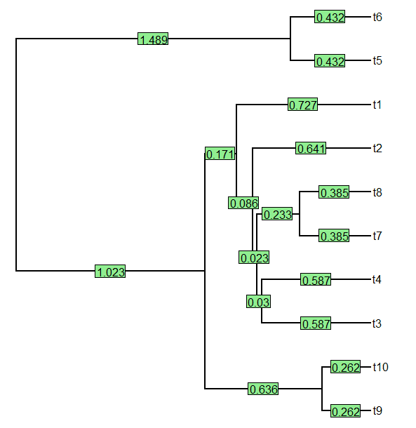
> ee
   t9   t10    t3    t4    t7    t8    t2    t1    t5    t6
0.262 0.262 0.587 0.587 0.385 0.385 0.641 0.727 0.432 0.432
> plotTree(tree)
> edgelabels(tree$edge.length)

Computing the residuals for individuals from phylogenetic regression

A little while ago I received the following query:

"To account for body size I used the phylogenetic regression of your phyl.resid function. I used the mean value of each trait per species. However, now I would like to plot the residuals against the ecological variables to show how they relate, including standard deviations for trait means. Is there a way to calculate phylogenetically corrected residuals with standard deviations? Or simply calculate residuals for more than one individual per species?"

Well, there are multiple ways we could go about doing this - with multiple possible solutions. The simplest thing, and the one I'd probably recommend for starters, is to fit the phylogenetic regression to x̄ and ȳ, the species means vectors; but then compute ŷ = [1 x]β and e = y - ŷ from the original data vectors, x & y.

Here's how that would look if we had input data vectors xi and yi, both with the same order but in which names(xi) and names(yi) contain only species names (& thus no unique identifiers):

## first aggregate xi & yi to compute species means
xbar<-aggregate(xi,by=list(names(xi)),FUN=mean)
xbar<-setNames(xbar[,2],xbar[,1])
ybar<-aggregate(yi,by=list(names(yi)),FUN=mean)
ybar<-setNames(ybar[,2],ybar[,1])
## now fit PGLS model
fit<-gls(ybar~xbar,data.frame(xbar,ybar),correlation=
  corBrownian(1,tree))
## compute yhat based on individual data in xi
yhat<-(cbind(1,xi)%*%fit$coef)[,1]
## compute individualized residuals
ei<-yi-yhat

Note that the species-wise mean of ei will be exactly equal to our residuals from the fitted model using species means. E.g., compare:

ebar<-aggregate(ei,by=list(names(ei)),FUN=mean)
ebar<-setNames(ebar[,2],ebar[,1])
## with
residuals(fit)

They should be the same.

That's it!